A²C² Magazine May 00 Vol. 3 No. 5 pgs. 13-16
Process Simulation of the Future
by
Jon Paul Van Buskirk, MSChE
Quality Monitoring & Control
Abstract
|
Computer aided process simulation has been increasingly popular in the last four decades. Advances in hardware and software applications driven by the demand of personal computing has had a positive influence on existing technologies. The need for both steady state and dynamic simulators in the chemical industry becomes greater as environmental, quality and safety issues grow with the expanding industries. Companies are beginning to recognize the benefits that simulators can provide including research and development, plant design and retrofitting, and plant operations. Coupled with modeling, control and optimization, simulation can enable companies to make better engineering and business decisions in both plant design and operations. As processes become more complex, incorporating varying degrees of automation, there is an increasing need in design and operations using simulators for process understanding. Modern analysis usually involves mathematical modeling either on a bench or pilot scale prior to a commercial plant. Two broad classifications include steady state and dynamic models. The attention to detail requires a solution based on the accuracy of the basic data obtained from scaled-down studies; therefore, steady state and dynamic simulators are highly effective when actual process data is used in physical property prediction, mass and energy balances, kinetics, transportation, etc. Process simulation leads to a deeper understanding of the internal mechanisms and characteristics of the process. |
Figure 1:
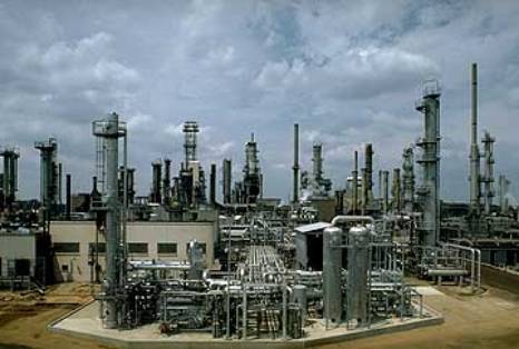
A Chemical Plant showing the diversity of equipment types
Overview
|
The Chemical Industry is diverse and requires several desktop tools for process understanding and improvement. Figure 1 shows the vast array and number of equipment in a common chemical process. Equipment is normally modeled on an individual basis or groups of common functionality. The number of model types and complexity is also diverse and modeling methods can range from a first principle approach to data intensive methods such as genetic algorithms or artificial neural nets. Data systems can range into the tens of thousands of variables and modeling methods based on this data is ultimately required to adequately represent these systems. A model representation is required for operations, control and optimization of the process. Modeling benefits include enhanced quality, safety, environmental, and economic controls. This article reviews several case studies leading to process improvement. These case studies are in reference to actual field applications and include: |
1. Steady-State Process Simulation
2. Dynamic Process Simulation
3. Detailed Equipment Design
4. Modified Iterative Measurement Test Method
5. Economic Optimization
| Various modeling methods are used in
these Case Studies. In all cases,
actual data is used as the basis for modeling.
This approach has proven to be the most reliable in all applications.
Any industry that uses data can benefit from this approach.
The advantage of this method is that a considerable amount of time can be
saved when data is available for modeling.
The ultimate requirement is that the model adequately represents the
actual system for prediction of future events.
Using actual data for this modeling basis will provide the most robust
results for these predictions.
Case
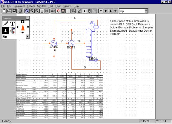
Study 1: A fundamental approach is required for new facilities design since data is not available. In the process industries, a simulator is used for mass, momentum, and energy balances and for chemical-physical property generation. The fluid components are selected, and the equipment and streams laid out in a flow sheet fashion. From this information, the simulator solves for the process conditions in a sequential method. The results provide the information necessary for equipment sizing, costing, predictive maintenance and optimization. Figures 2 and 3 are typical depictions of process flow sheets by the steady-state simulator from Design II for Windows™. Figure 2 depicts a simulator for rigorous process design of a refinery. Figure 3 is an example of a debutanizer column design. One objective of a simulation may be to design and optimize process operations to maximize energy savings. |
Figure 2:
Depicts a simulator for rigorous process design of a refinery
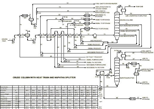
Figure 3:
An example of a debutanizer column design
Case
Study 2:
Facilities Design using a Dynamic Simulator:
|
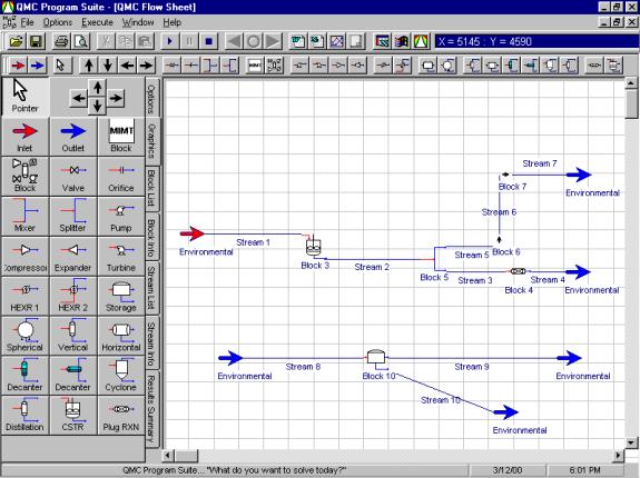
Dynamic transitions in chemical processes cannot be accurately modeled using a steady-state simulator. For all practical purposes, a dynamic simulator integrated with a full physics package based on a time dependent method should be used for transitional data analysis. As with the steady-state simulator dynamics must include all physical/chemical property calculations with a flow sheet generator interface. Figure 4 is an example of a simplified flow sheet of a reactor system the utilizing QMC DYFLO Program for reactor kinetics. The model is in a dynamic time domain and can also be used for tanks, pumps, compressors/expanders, heat exchangers, pipes & valves, control valves, controllers, reactors/combustors, distillation, etc. The technology has been successfully used in chemical processes for over 30 years with many benefits for system analysis and robust methods for actual operational evaluation of steady-state and transitional conditions. |
Figure 4:
An example of a simplified flow sheet of a reactor system
utilizing the
QMC DYFLO for reactor kinetics
Case
Study 3:
Facilities Design using Detailed Sizing Programs:
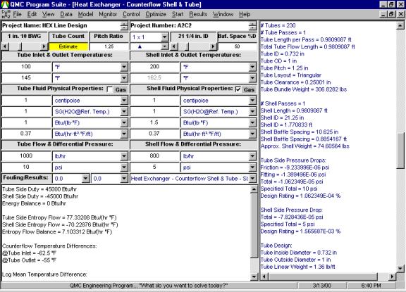
| From steady-state and/or dynamic simulation, a detailed design of equipment can be reviewed and verified. In the Chemical Industry, this equipment includes piping, control valves, safety valves, flow meters, pumps, compressors, heat exchangers, decanters, gas-liquid separation vessels, etc. Figure 5 provides the results of a control valve sizing procedure. Depicted is the control valve flow coefficient, termed CV, versus flow rate. Also shown is the limit of flows for this control valve system. Figure 6 is a detailed design program to size a Counterflow Shell and Tube heat exchanger. Detailed equipment design typically gives thorough results, i.e. mechanical design, stress analysis, etc., for final design generating spec sheets for the vendor. |
Figure 5:
Results of a control valve sizing procedure
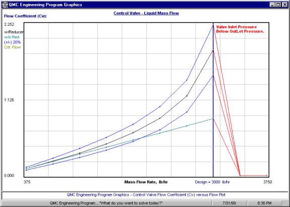
Figure 6:
A detailed design program to size a Counterflow Shell and Tube
heat
exchanger
Case
Study 4:
Modified Iterative
Measurement Test Method:
| An
enhancement to simulation in order to determine the measured data accuracy is
the Modified Iterative Measurement Test Method (Serth and Heenan, AIChE Journal,
32 p. 733, 1986). The QMC MIMT
Program solves the linear and non-liner
data-reconciliation/gross-error-detection problem.
For a given set of measured data, the program generates a reconciled data
set, i.e., one, which is consistent with all applicable constraints, such as
material balance or model based requirements.
It also generates a list of measurements, which are suspected of being
grossly in error, as well as estimates of the correct values of the suspect
measurements. Typical applications
include total material balances, temperatures, pressures, etc. for chemical
processes or plants, steam-metering systems in plants and refineries, and
natural gas distribution systems. However,
the program is applicable to any data set for which the measured variables are
related to one another by a system of linear or non-linear algebraic equations.
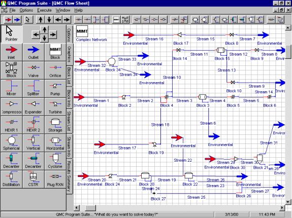
Complex networks of pipes, tanks and process components are shown in
Figure 7. |
Figure
7:
Complex networks of pipes, tanks
and process components
Case
Study 5:
Economic Optimization:
|
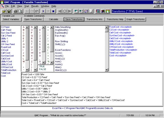
Economic reporting provides a procedure to monitor and optimize production costs. The steps are: a) Perform economic balance, b) Model economics using plant data, and c) Minimize production costs using a model optimizer. Economic optimization and reporting can run in on-line and off-line modes. The economic balance can be done using spreadsheet functions or a transform calculation program. The transform calculations should use both fixed and variable costs for a more complete economic evaluation. This procedure is shown in Figure 8. Provided in this figure are the Plant data, calculated economic variables, and associated economic equations. Results are saved to a spreadsheet for future analysis. For this example a small part of the total process, a reactor system, is used for economic analysis. This approach allows focus to different operating areas and allows for localized optimization of individual unit operations. A global approach will help select which areas of the plant will provide the major profit improvement. The global approach will also provide a monitoring check on realized production cost savings. Figure
8: |
|
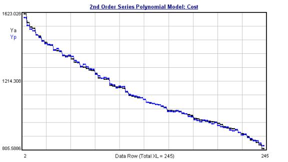
The (sorted) cost per hour is given in Figure 9. As shown on this graph, a wide range of operating costs exists. This is due to a wide range in production rates and the effects of fixed and utility costs. For this process, it is best to maximize production rates to minimize product costs. A model of the cost can include applicable process data such as pressures, temperatures, flows, and concentrations. The model can then be adjusted to minimize the cost with respect to these variables when used as system set points. The results of this modeling procedure are also shown in Figure 9 (where Ya are the actual values and Yp are the model-predicted values for cost per pound of production.) Figure 9: Results of a modeling procedure |
|
With this model, many methods are available for optimization. This provides the set points that minimize costs. This can be done for both on-line and off-line applications. In this case, the optimum occurs at maximum production rates. However, this maximum production may be limited by several factors, such as hardware, raw materials availability, or off-site limitations. Therefore, a constrained optimization algorithm should be utilized. Other modeling methods to be considered include genetic algorithms, neural net, evolutionary, etc., or simulation methods adapted towards the respective industry. The modeling technique selected should come with an optimizer that can handle a wide range of applications. The maximum benefits of modeling are when an optimization procedure can be utilized. Conclusion: This article reviewed several case
studies involving design, simulation, data reconciliation and optimization. These technologies provide a basis leading to process
improvement. These case studies are
in reference to actual field applications and include: Steady-State Process Simulation,
Dynamic Process Simulation, Detailed Equipment Design, Modified
Iterative Measurement Test Method and Economic Optimization. It was also shown how simulation, modeling and optimization methods work together in a unified approach to design and improve any process. When these methods are used for auditing, control, and optimization improvements, a quality, safety, environmental, and economic advantage can be obtained by operating at peak performance levels. The applications of these techniques are not limited to the process industries. They can be adapted to any industry that has data systems including contamination control and critical cleaning. Implementation will provide a definite technology advantage, and promote a logical and systematic approach for continuous improvement. |
_________________________________________
| Jon Paul Van Buskirk is a Principal with Quality Monitoring & Control. He has experience in refineries, petrochemical and polymer industries and may be reached at QMC@QMC.net. |
